Agenda
- Data standardization (encoding) for data input
– Binary
– Positive-Negative
– Manhattan & Euclidean
– Categories encoding - Standardization vs. Normalization
– Min-Max Normalization
– Gaussian Normalization - Data Decoding
– Softmax activation function
– Mean Squared Error
– Entropy (Information Theory)
– Mean Cross Entropy - MSE vs. MCE
This article assumes you have a pretty good knowledge about Neural Networks and some basic algorithms like Backpropagation.
When you work on neural networks, you always see yourself dealing with numeric data, basically, neural networks can be performed only with numeric data, algorithms such as backpropogation or when you simulate perceptron, you always use some functions or equations to calculate your output, when you build your network you use matrices to represent the biases and layer-to-layer values, after you get the output, you estimate the error and try to get the most optimal solution. As you see, you always use numeric data.
But, what about the other data types?.. Could neural networks be built to make a good prediction or get an optimal output given data like “food”, “location” or “gender”?
The solution is to encode the non-numerical data and normalize it to be represented as numeric data, this operation is called “Data Encoding and decoding”, the name “Data Standardization” is used too. Suppose your input data looks like “ID”, “Name”, “Nationality”, “Gender”, “Preferred food” and “Wage”, for more clarification, the following table represents a training set, each ith row represents ith person.
ID Name Gender Nationality Preferred food Wage
1 Hani Male French Rice 30
2 Saad Male Italian Pizza 40
3 Sofia Female Russian Spaghetti 15
To make it easy, I will represent the above table in a simple 2D matrix

I will take each column, then check if it contains numeric data or not.
The first column is “ID”, the ID is just considered to be a unique identifier for each item in the training set, so this column isn’t involved in the process.
The second column is about person’s name, it isn’t involved in the process too, but you need to map each ID with the name and use ID instead of the name to avoid duplicated names in the training set
The third column is about the Gender, obviously, the Gander type has only 2 values, Male or female, you have 3 ways to encode this data
- 0-1 Encoding (Binary method)
– You are free to choose, male will be set to 0 and female will be set to 1 or the vice versa - +1 -1 Encoding
– If you find yourself you will be in trouble if there is a 0 value in your input, use +1 and -1 values instead - Manhattan Encoding (x-y axis)
– Simply, use pair of values, this method is good when you deal with more than 2 values, in our case Gender we set the male by [0, 1] and female by [1, 0] or the vice versa, this method will work perfectly with 4 possible values, if there are more than 4 possible values, you can include -1 in your encoding, this will be called Euclidean Encoding.
The fourth column which represents the person’s nationality, there is no known approach or method to deal with this kind of types, person’s nationality is represented as a string value, some of you could encode each of the characters string to ASCII then use some constant to normalize the data, but the method I prefer which gives me flexibility when I work on this kind of data is using matrices.
Matrices approach depends on the size of possible values of the category, so, first of all we count the number of different values in the column. Back to our training set, we will see there are only 3 nationalities presented in the table, let’s create a matrix N that will hold the column values, the size of matrix is m x 1, m is number of different values in the input data, in our case m = 3.

We will create a new identity matrix A of the same size of N

Let N = A.

Now we will set each nationality values to its corresponding row, thus
French = [1, 0, 0].
Italian = [0, 1, 0].
Russian = [0, 0, 1].
The only one thing remaining is to replace each nationality string to its corresponding vector value.
This approach works perfectly with small and medium input data, and works good with large amount of input data.
Pros:
- Dynamic
- Easy to understand
- Easy in coding
Cons:
- Memory
- Complicated when dealing with very huge amount of data
- Bad performance with huge amount of data
The fifth column is about the preferred food for each person, this will be treated like the previous column, the matrices approach and count the number of different food in the input. There are some special cases could be found in this column if it is given in other input data, we will talk about it in another post.
The last column is the wage, as you see this column is already using numeric data to present the wage value per day of each person (you don’t say!), Will we leave the values without do any processes on it?, the answer is no, we shall normalize these values to suit the other previous values, experience shows that normalizing numeric data produces better output than leaving them without normalization, but how will we normalize these values?
Before we answer this question, we need at first know exactly the difference between “Normalization” and “Standardization”.
The relation between Normalization and Standardization looks like the relation between Recursion and Backtrack, any Backtrack is a Recursion, but not any Recursion is considered to be a Backtrack. Any Standardization is considered to be Normalization, but not any normalization is considered to be Standardization, to clarify more, we need to know the definition of each one of them.
In statistics, commonly normalizing data is to set the value within 1, the value should only be in these intervals [0, 1] or [-1, 1], for example in RGB, the basic value for each color is from 0 to 256, the values could be 55, 40, ..etc., but it can’t exceed 256 or gets below 0, we want to normalize the colors values to be in the interval [0, 1]. The most common method for normalization is.
- Min-Max Normalization
In Min-Max normalization, we use below formula

The resulted value won’t exceed 1 or get below 0, you can use this method only if you want to set a value in range [0, 1].
In [-1, 1] we use the below formula if we want to make 0 centralized

Standardization is pretty the same thing with Normalization, but using Standardization will calculate the Z-score, this will transform the data to have 0 mean and 1 variance, the resulted value will be relatively close to zero according to its value, if the value is close to the mean, the resulted value will be close to zero, it is done using Gaussian normalization equation.

Check the following figure (from Wikipedia):-

As you see, there isn’t much difference between Standardization and Normalization, experience shows that using Gaussian normalization gives better output than Min-Max normalization.
Back to our table, as I have said, it will be better if we use standardization with numeric values of “Wage”, I will use Gaussian normalization.
Step 1:

Step 2:

Step 3:
Take each wage value and use Gaussian normalization equation

As you see, the result is 0.09 which is near zero because the value “30” is very close to “28.33”, in addition the value is positive because the wage value is more than mean, if the value was less than 28.33, the normalized value will be negative, that’s why Gaussian normalization is better Min-Max, Gaussian normalization gives you more information about the true value.
Now, let’s put all the above together and get the normalized input data to use it in the neural network

Data Decoding
All we have done till now is just about normalizing the input data and using some encoding techniques to transform a category type value to numeric to suit neural networks, but what about the output? .. Obviously, the output of encoded input will be in encoded form too, so.., how we can get the right prediction or classification to the output? In other words, how can we decode the output to their original form?
The best way to understand what we will do next is by example, from our previous table; we set an encoded value to each nationality
French = [1, 0, 0].
Italy = [0, 1, 0].
Russia = [0, 0, 1].
Assume that you get sample output like that [0.6, 0.3, 0.1], [0.1, 0.7, 0.2], [0.0, 0.3, 0.7], for the targets French, Italy and Russia respectively, how do you check the validation for this example?
In this case, you can think the values of each vector as a probability, you can assume that when the values are in range [0, 1] and the sum of all vector values is equal to 1, from this assumption we could easily get the right prediction of the output.
Output Natio.
[0.6, 0.3, 0.1] [1, 0, 0]
[0.1, 0.7, 0.2] [0, 1, 0]
[0.0, 0.3, 0.7] [0, 0, 1]
Check each value of the output with its corresponding value in nationality’s vector; you could see in the first case, the value “0.6” is the closer value to 1 than “0.3” and “0.1”, which shows that it is a right prediction. The same with the second and third cases, we can conclude that the output makes a good prediction.
We can use the previous approach when the values of the output vector are within [0, 1], but what can we do with outputs like [3.0, 2.5, 7.0], all the values is greater than 1, you can’t use the previous method with this, so, what shall we do?
The solution is to use the softmax activation function, using it will transform your output values to probabilities, these new values must be between [0, 1], the formula is.

Let’s calculate the new vector using the above equation
Step 1:

Step 2:

So, the new output vector is [0.017, 0.010, 0.971], now you can use this vector for your classification
There is a lot of math behind softmax function; you can search about it if you are interested.
def softMax(self, output):
    newOutput = [0.0 for i in range(0, self.numberOfOutputs)]
    sum = 0.0

    for i in range(0, self.numberOfOutputs):
        sum += round(output[i], 2)

    for i in range(0, self.numberOfOutputs):
        newOutput.append(output[i] / sum)

    return newOutput
Errors
All our assumptions till now depends on that the neural network output will be always correct, the output will always match the target output, but practically this isn’t always true, you may face something like
Output Target.
[0.3, 0.3, 0.4] [1, 0, 0]
According what we have said and the method we have used, the last value in the output vector is the nearest value to 1, but this isn’t matched with our target vector, we conclude from that there is an error with the prediction or classification, it is important to compute your output error, this will help to improve your neural network training and to know how the efficiency of your network, To compute the value of this error, there are 2 common approach:-
- Mean Squared Error
- Mean Cross Entropy
We will talk about each one of them; let’s begin with Mean Squared Error (MSE)
From Wikipedia, the definition of MSE is “the mean squared error (MSE) of an estimator measures the average of the squares of the “errors”, that is, the difference between the estimator and what is estimated. MSE is a risk function, corresponding to the expected value of the squared error loss or quadratic loss.”
That is, let’s create the some training items and the supposed target values
Output Target.
[0.3, 0.3, 0.4] [1, 0, 0]
[0.2, 0.3, 0.5] [0, 1, 0]
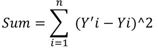
First, let’s get the sum of the squared difference between the 2 vectors values of the first training item

The second training item

Finally, let’s get the average of these sums

As you see, the error is high, indicates that the prediction is very far from the correct one; this should guide you to train your network more.
Let’s see the other approach which I prefer more, Mean Cross Entropy (MCE), before we get working with examples, I would like to get into the “Entropy” concept, so, if you get bored with that, you can ignore it and jump to the MCE equation and example.
In Information Theory, Quantification is a concept that indicates the amount of information that you can gain from an event or sample, the amount of information reflects on your decisions, assume that you are creating a system that deals with data send/receive, for example Skype, you send data (speech) and receive data, how do you determine the best encoding method to deal with these voice signals?, you decide that when you know information about the data, for example if your input data will be only “Yes” or “No”, you can use only 1 bit to encode this case, so, we can say that the Entropy of this case is 1 which is the minimum number of bits needed to encode this case. There is other kind of information you could obtain from an event like its probability distribution which I will focus in.
So, Entropy is the key measurement to know the average number of bits to encode an event, we can obtain from that the more information we can get from an event the more Entropy value we will expect,
As I said before, probability distribution of an event is considered to be good information we can use Entropy to evaluate this probability distribution, Entropy result evaluates the randomness in the probability distribution, this evaluation is very important in the case you want to get the most optimality from a uniform distribution, assume that you have variables X, Y which have actual distribution [0.3, 0.2, 0.1, 0.4], [0.5, 0.5] respectively, to calculate the Entropy of X, E(X) we use


As you see, in the first distribution X, the Entropy is 1.85, and 1 in Y, this because the randomness in X distribution is higher (more information) than Y (less information).
You can use Entropy to compare between two or more probability models, this comparison shows you how close or how far between these models with your target model, assume that you have a variable T which has actual probability distribution [0.2, 0.1, 0.7], and you have 2 probability models X and Y, which have probability distribution of [0.3, 0.1, 0.6] and [0.3, 0.3, 0.4] respectively, , you want to get the nearest or the closet model to your target model T, the first step is to calculate your target’s Entropy

The second step is to calculate the Cross Entropy (CE), CE is a variant of Entropy function, which estimates how close of model B with model A

Let’s estimate how close model X to model T

Model Y with T

We can observe from that model X is much closer to T than model Y.
There are many other variants of Entropy, I only mentioned that the ones you may use as a programmer in your applications, if you are interested with Entropy as key concept of Information Theory, you can search about it, you will find good papers talking about it.
Mean Cross Entropy (MCE) is my preferable approach when computing error in the neural network categories output, I will use the same example of MSE.
Output Target.
[0.3, 0.3, 0.4] [1, 0, 0]
[0.2, 0.3, 0.5] [0, 1, 0]
MCE measures the average of how far or close the neural network output with the target output, MCE formula is the following

Let’s begin with the first training item

The second training item

MCE calculation,

Your target is to reach 1, and the MCE is 1.7, this indicates that there is a 0.7 error
If you find yourself didn’t understand well, please go above where you will find all information you want to fully understand MCE approach.
MCE vs. MSE
Well, in machine learning the answer is always “it depends on the problem itself”, but the both of them effect on the gradient of the backpropagation training.
Here is the implementation of the both methods
def getMeanSquaredError(self, trueTheta, output):
    sum = 0.0
    sumOfSum = 0.0;

    for i in range(0, self.numberOfOutputs):
        sum = pow((trueTheta[i] - output[i]), 2)
        sumOfSum += sum;

    return sumOfSum / self.numberOfOutputs
def getMeanCrossEntropy(self, trueTheta, output):
    sum = 0.0

    for i in range(0, self.numberOfOutputs):
        sum += (math.log2(trueTheta[i]) * output[i])

    return -1.0 * sum / self.numberOfOutputs
References
Stanford’s Machine Learning Course
http://en.wikipedia.org/wiki/Entropy_(information_theory)
http://www.faqs.org/faqs/ai-faq/neural-nets/part2/section-7.html
James McCaffrey Neural Networks Book

One thought on “Data Normalization and Standardization for Neural Networks Output Classification”